We are really proud of the immunoSEQ Analyzer — it’s a great tool with a ton of charts and visualizations specifically tareted at immunosequencing. And since the field is new to many folks, it’s great to have an environment where we can share the approaches and techniques we’ve developed over the years. If you’re an Adaptive customer and you’re not using it — you’re missing out.

But at the same time, there are a zillion analysis and visualization tools out there, and each of them has their own strengths. Our goal is to make sure that immunoSEQ data shines in all of those environments, because better tools == faster discoveries == better treatments for real people.

I’m really excited today to show off our latest such integration. “rSEQ” is an installable package that makes it super-easy to work with immunoSEQ data with R. You can read all the gory details in this technote (free Analyzer login required), and I’ll walk through a simple example here so you can get an idea of just how awesome it is.

You’ll need the popular devtools package in order to install rSEQ. The technote provides some details on this, but in its simplest form all you need to do is:

Now you’re ready to create an authenticated session to immunoSEQ. For this, you’ll use the same credentials you use to log into the web site; as in:

For this demo, though, we’ll use the public immunoSEQ demo account — so even if you don’t have your own immunoSEQ account, you can follow along:

We hold onto that “rseq” variable because it’s the token that we’ll use in future calls into immunoSEQ. Now let’s look at a few calls:

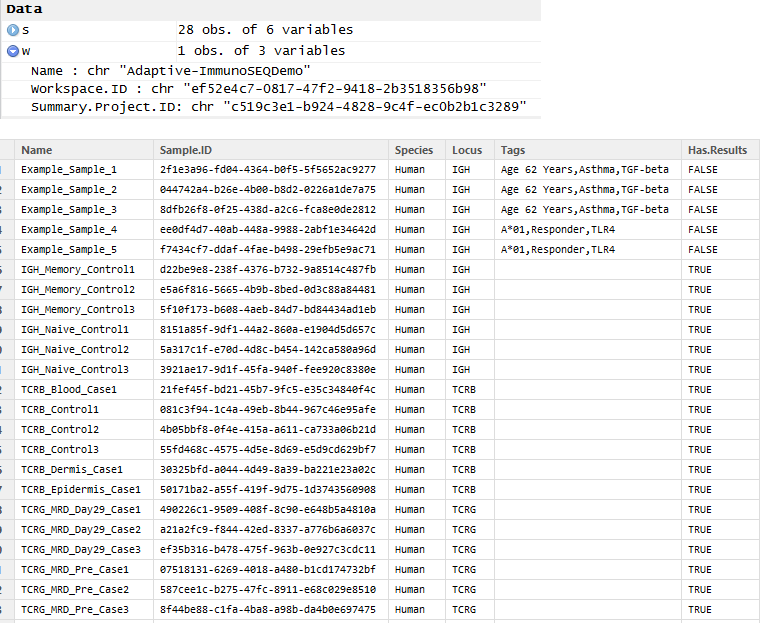
Snipping from my RStudio environment window, you see that w and s both contain data frames. w lists all the workspaces I have access to (just one for the demo account), and s is the list of all samples in that workspace (the rSEQ_samples call takes a workspace ID, which I’ve cut out of the workspace data frame above).

Once I have samples with results, I can fetch the actual sequence data for those samples, and pretty easily do some neat things. One of our most common real-world use cases is tracking “minimum residual disease” in blood cancers — in short, identifying the dominant clones in a pre-treatment sample, then watching post-treatment to make sure that clone is (mostly) gone. Our demo workspace includes a few MRD cases, so let’s build a really simple clone tracker that identifies those dominant clones and then shows before and after values.

To be sure, this is a simplistic and only marginally-useful example — it only includes one “after” sample, and uses a very naïve threshold to decide what is “dominant.” But nonetheless, it’s a pretty sweet example of what you can do with immunoSEQ data in R with a VERY small amount of code.

First, let’s download the sequence data for a pair of before and after sequences. I’ll cut out sample IDs by name to do this:

These guys are downloading a lot of data, so be patient! (Fun exercise for the reader — why does seqMRD take so much longer to download than seqDiag? I’m not telling, you’ll have to figure that out for yourself.)

Go ahead and take a look inside these guys … there is a TON of useful information in there, ranging from the nucleotide and amino acid strings, to V and J gene usage, N insertions, and much more. These are the same columns that our “Sample Export” feature returns.

Right away, you can do some neat things; try a species histogram of CDR3 lengths for the Diagnostic sample:

Pretty neat. But back to MRD. What we’re interested here is just finding the clones that make up more than 5% of the repertoire pre-treatment. Paste this function into your R session:

  cloneTracker = function(seqDiag, seqMRD, thresholdPct) {
    diags = seqDiag[seqDiag$frequencyCount.... >
      thresholdPct,c("nucleotide","frequencyCount....")]
    track = merge(diags, seqMRD, by = "nucleotide")
    track = track[,c("nucleotide","frequencyCount.....x","frequencyCount.....y")]
    ct = t(data.matrix(track[,2:3]))
    colnames(ct) = track[,1]
    rownames(ct) = c("Diag","MRD")
    attr(ct, "thresholdPct") = thresholdPct
    return(ct)
  }


Then call it, passing in your sequences and a threshold of 5%:

This function first selects out the relevant clones from the diagnostic sample, joins those rows with the MRD sample and then massages them into a simple table that shows before and after frequencies for all identified clones (two in this case):

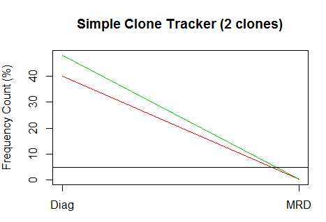
Cool! Even better is showing these guys in a simple time series plot, using this function:


  plotCloneTracker = function(ct) {
    plot.ts(ct, plot.type="single", col=2:(ncol(ct)+1), axes=FALSE,
      ylab="Frequency Count (%)", xlab="",
      main=paste("Simple Clone Tracker (",ncol(ct)," clones)",sep=""))
    box()
    axis(2)
    axis(1, at=1:2, lab=c("Diag","MRD"))
    abline(attr(ct, "thresholdPct"), 0, col=1)
  }

And of course, call it:

FANCY! And in case it’s not obvious, I’m no R virtuoso by a longshot. I am really, really excited to see what our research customers can do with this stuff. Have a great function or plot? Let me know and I would love to share it here.

So. Much. Fun. And just wait until you see what’s coming next. Until then!