
Faced with the daunting task of saving $6.5 million in annual spend at a large aerospace manufacturer, our small team began evaluating options. We first examined the usual suspects, such as SKU rationalization, improved repair/refurbishment practices, and optimized preventative maintenance to reduce unnecessary equipment downtime. Little did we know at the time, but our most significant savings would be found in using statistical models to optimize the stocking level of each spare part held in inventory.
There is a trade-off between the carrying cost of inventory and the risk of downtime if spare parts are unavailable when needed. If too many spare parts are held, the prices of financing, insurance, taxes, physical handling, warehousing, etc. will balloon. On the other hand, if too few spare parts are held (especially those with long lead times), the cost of equipment downtime could be enormous. This trade-off is illustrated in the following chart:
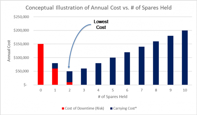
*Carrying cost includes the costs of financing, warehousing, physical handling, taxes, insurance, obsolescence, deterioration, and pilferage.
As one can see in this conceptual illustration, the optimal stocking level is two (2) spares, since that number has the lowest annual cost when balancing the cost of downtime and carrying cost. The challenge here is that each part will have a different optimal stocking level based on that part’s unique characteristics. These characteristics may include the part’s lead time, the criticality of the machine on which the part is used, whether that machine has redundancy or is a single point of failure, etc.
While this approach seemed plausible at first, we then discovered that our aerospace client had over 50,000 different spare parts SKUs in the system. Imagine performing a detailed analysis on a part-by-part basis for over 50,000 different parts! While I’m not afraid of working late nights at the hotel, this level of effort would have been entirely unrealistic.
This is where using an algorithm to identify each part’s target stocking level (TSL) came into play. We started with a standard formula for stocking level:
Stocking Level = Cycle Stock + Safety Stock
In this case, cycle stock is the lead time demand — i.e., how many spares we expected to use within the time needed to replenish the stock. This was quickly determined by examining a part’s lead time and historical demand frequency.
Safety stock is the additional inventory needed to ensure that we don’t run out in periods where more than expected demand occurs. This is much more difficult to calculate. In his excellent article on safety stock, Peter L. King describes three different safety stock formulas (all three shown below) to use depending upon the circumstances. [i]
Which formula should be used?
According to King, when both demand variability and lead time variability are 1) necessary, 2) independent, and 3) normally distributed, we should select the formula shown below:
![]()
However, when demand and lead time variability are not independent, safety stock should be the sum of the two individual calculations, as shown below:
![]()
Unfortunately for us, actual historical lead time was not captured in the system. We knew the expected lead time for each part but did not have visibility into the actual lead times over the past few years. Since we were unable to calculate historical lead time variability, we focused on demand variability and used the simplified equation shown below:


While it is preferable to use the lead time variability if the data is available, not having this data was not a significant concern because the demand variability is the key driver of how much safety stock is needed.
More information on each argument in the equation and the reasoning behind it can be found in Peter King’s article here.
We also realized that increasing our service level (in this case, having a spare part available when needed) from 90% to 99% would require an exponential increase in safety stock as we moved up. To balance the service level with the carrying costs, we categorized each part by criticality—based upon the criticality of the equipment on which the part was used. We then assigned an appropriate service level for each criticality level. For example, we gave each part a criticality score from Low to Extra High and assigned service levels accordingly, as shown below. The Z-score is the corresponding value (statically, the number of standard deviations to the right of the mean in a normal distribution) required to attain the desired service level.
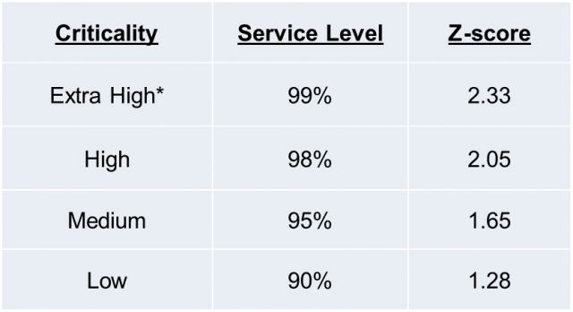
*Reserved for parts used on “single point of failure” equipment
Criticality was driven by the impact of having a specific machine down. For example, if a machine were a single point of failure or a bottleneck in the production process, the criticality was much higher than for a device with excess capacity or redundancy.
To estimate the desired service level by criticality, we started with intuition and experience, but then refined our numbers based on an effective formula provided by Joannès Vermorel. According to Vermorel, we can estimate the optimal service level as follows:
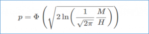
Where:
p = the service level
Φ = the cumulative distribution function associated with the normal distribution
M = the total per unit stockout cost, and
H = the per unit carrying cost for the duration of the lead time
For more information on each argument in the equation and the reasoning behind it, please refer to Joannès Vermorel’s article here. [ii]
Once the component formulas were selected, it was then a matter of combining them into a master algorithm to be used across all parts, downloading the inventory data from the system into a spreadsheet, writing the algorithm into the spreadsheet, and calculating the optimum level of stock for each part.
Once we had determined the TSL for each part, the final steps included dispositioning excess inventory where needed and purchasing additional inventory where required. Tip: if a component with excess inventory is used frequently and has low resale value, it is often best to consume that inventory over time (and delay the replenishment in the near term) rather than trying to sell that inventory on the open market. The chart below illustrates where to reduce or add stock by part, based upon the calculated TSL:
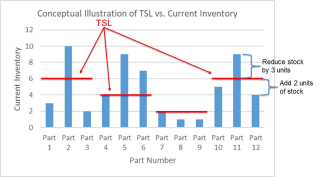
As we can see in the illustration above, Part 11 should be reduced by three parts, while Part 12 should be increased by two parts. This will save carrying costs for Part 11 while reducing the risk of downtime for equipment using Part 12.
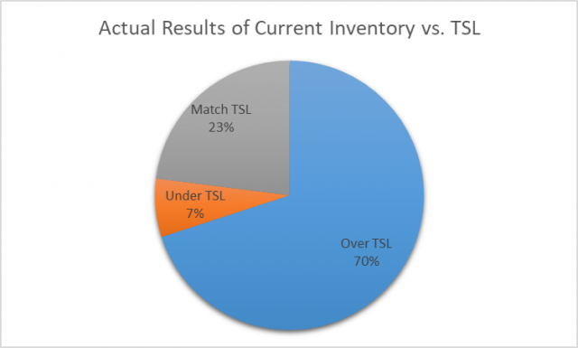
Across all part numbers for which we had sufficient data to run the algorithm, we found that most often, there were more parts in current inventory than needed. However, we did find that 7% of the part numbers had a lower inventory quantity than required. Surprisingly, when we looked at six recent requests from managers to order more inventory, all six of the part numbers requested fell within that 7% sliver of parts for which our current list was under the TSL. While statistically insignificant due to the small sample size, this discovery did boost our confidence in the algorithm’s practical benefits.
By using the strategy described above, we were able to identify $4.9 million worth in annual savings to the company — which would be realized over time as we lowered carrying costs while simultaneously reducing the risk of equipment downtime. With such a high ROI in such a short time, many companies would have a great deal to gain from following a similar exercise.
Citations
[i] Source: King, Peter L., “Crack the Code; Understanding Safety Stock and Mastering Its Equations,” APICS Magazine, July/August 2011, http://web.mit.edu/2.810/www/files/readings/King_SafetyStock.pdf
[ii] Source: Vermorel, Joannès, “Optimal Service Level Formula (Supply Chain),” January 2012, https://www.lokad.com/service-level-definition-and-formula